Probabilistic Proofs (Shannon)
This is an active WIP from #899 that is merge in for public iteration
tl;dr Probabilistic Proofs is a method to scale Pocket Network indefinitely.
Abstract
This document describes the mechanism of Probabilistic Proofs, which is what allows Pocket Network to scale verifiable relay throughput to match an arbitrarily large demand. Precisely, it allows an unlimited number of "sessions" which pair (Applications and Suppliers for a given Service) by requiring the creation of a single on-chain Claim for each such session, but only probabilistically requiring an on-chain proof if it's total reward amount is below a specific threshold.
External stakeholders (i.e. DAO/Foundation) need to be involved in adjusting the
ProofRequirementThreshold by statistically analyzing onchain data, along with selecting
an appropriate ProofRequestProbability that balances scalability and security. In turn, these values
are used to derive on-chain reward and penalty amounts for honest and dishonest Suppliers, respectively.
The penalty amount is then used to derive SupplierMinStake.
Reasonably selected values can be chosen to easily scale the network by 100x without compromising
security.
The results show that choosing a value of 20 POKT for ProofRequirementThreshold,
the 95th percentile of all Claims, along with a ProofRequestProbability of 0.01,
can enable 100x scalability of the network if the Slashing penalty for invalid/missing
proofs is set to 2,000 POKT. As long as the minimum required stake for Suppliers exceeds
this value, staked collateral will be available for slashing, if needed.
In future work, we will look at a potential attack vector that still needs to be considered, along with further research on the topic.
Table of Contents
- Relationship to Relay Mining
- Problem Statement
- Example Scenario
- High Level Approach
- Key Question
- Guarantees & Expected Values
- Modeling an Attack
- Defining a Single (Bernoulli) Trial
- Conceptual Parameters: Onchain, Modeling, Governance, Etc
- Dishonest Supplier: Calculating the Expected Value
- Modeling a Dishonest Supplier's Strategy using a Geometric PDF (Probability Distribution Function)
- Expected Number of False Claims (Failures) Before Getting Caught (Success)
- Modeling a Dishonest Supplier's Strategy using a Geometric CDF (Cumulative Distribution Function)
- Total Rewards: Expected Value Calculation for Dishonest Supplier Before Penalty
- Expected Penalty: Slashing amount for Dishonest Supplier
- Total Profit: Expected Value Calculation for Dishonest Supplier AFTER Penalty
- Honest Supplier: Calculating the Expected Value
- Setting Parameters to Deter Dishonest Behavior
- Example Calculation
- Generalizing the Penalty Formula
- Considering false Claim Variance
- Crypto-economic Analysis & Incentives
- Conclusions for Modeling
- Morse Based Value Selection
- TODO_IN_THIS_PR: Above Threshold Attack Possibility
- Future Work
Relationship to Relay Mining
I think it may be worth noting that while probabilistic proofs reduce the number of on-chain proofs (block size), it will drive up supplier min stake amount as it's scaled. I think relaymining helps to mitigate this by taking the scaling pressure off of probabilistic proofs by reducing the size of each proof. Additionally, relaymining has the effect of minimizing the "max claim persistence footprint size":
Problem Statement
tl;dr Too many on-chain Proofs do not scale due to state bloat and excessive CPU usage.
The core limiting factor to Pocket Network's scalability is the number of required on-chain Proofs. For details on how Proofs are generated and validated, see the Claim & Proof lifecycle section.
For every session (i.e. (Application, Supplier, Service) tuple), it is possible to construct a
Merkle Proof which proves the Claimed work done, which can be stored on-chain.
These Proofs are large and costly to both store and verify. Too many Proofs result in:
- State Bloat: Full Node disk space grows too quickly because blocks are large (i.e.,full of transactions containing large Proofs), increasing disk usage.
- Verification Cost: Block producers (i.e. Validators) MUST verify ALL Proofs (once), correlating average CPU usage with the average throughput of on-chain Proofs.
There is a lot of research around this type of problem, but our team is not actively
looking into 0-knowledge as a solution at the time of writing (2024).
TODO_IN_THIS_PR: Reference the papers from justin taylor, Alin Tomescu, and axelar (avalanche?).
Example Scenario
Consider the hypothetical scenario below as an extremely rough approximation.
TODO_IN_THIS_PR: Turn this into a table.
Network parameters:
- Session duration:
1hour - Number of suppliers per session (per app):
20 - Number of services per session (per app):
1
Network state (conservative scenario):
- Number of (active) services:
10,000 - Number of (active) applications:
100,000 - Number of (active) suppliers:
100,000
Assumptions for the purpose of an example:
- Median Proof Size:
1,000bytes - Total time:
1day (24sessions)
Total disk growth per day:
10,000 apps * 1 Proof/(service,supplier) * 20 suppliers/app * 1 services/session * 24 sessions * 1,000 bytes/Proof = 4.8 GB ≈ 5 GB
CRITICAL: A very simple (conservative) scenario would result in 5 GB of disk growth per day, amounting to almost 2 TB of disk growth in a year.
This discounts CPU usage needed to verify the Proofs.
High Level Approach
tl;dr Require a Claim for every (App, Supplier, Service) tuple, but only require a Proof for a subset of these Claims and slash Suppliers that fail to provide a Proof when needed.
The diagram below makes reference to some of the on-chain Governance Params.
Key Question
What onchain protocol governance parameters need to be selected or created to deter a Supplier from submitting a false Claim? How can this be modeled?
Guarantees & Expected Values
Pocket Network's tokenomics do not provide a 100% guarantee against gaming the system. Instead, there's a tradeoff between the network's security guarantees and factors like scalability, cost, user experience, and acceptable gamability.
Our goal is to:
- Model the expected value (EV) of both honest and dishonest Suppliers.
- Adjust protocol parameters to ensure that the expected profit for dishonest behavior is less than that of honest behavior.
A Supplier's balance can change in the following ways:
- ✅ Earn rewards for valid Claims with Proofs (Proof required).
- ✅ Earn rewards for valid Claims without Proofs (Proof not required).
- 🚨 Earn rewards for invalid Claims without Proofs (Proof not required).
- ❌ Get slashed for invalid Proofs (Proof required but invalid).
- ❌ Get slashed for missing Proofs (Proof required but not provided).
The goal of Probabilistic Proofs is to minimize the profitability of scenario (3🚨) by adjusting protocol parameters such that dishonest Suppliers have a negative expected value compared to honest Suppliers.
Modeling an Attack
Defining a Single (Bernoulli) Trial
We use a Bernoulli distribution to model the probability of a dishonest Supplier getting caught when submitting false Claims.
- Trial Definition: Each attempt by a Supplier to submit a Claim without being required to provide a Proof.
- Success:
- A dishonest Supplier gets caught (i.e. is required to provide a Proof and fails, resulting in a penalty)
- Taken from the network's perspective
- Failure:
- A dishonest Supplier does not get caught (i.e. is not required to provide a Proof and receives rewards without providing actual service)
- An honest Supplier is rewarded
- All other outcomes
- Does not include short-circuited (i.e. Claim.ComputeUnits > ProofRequirementThreshold)
Conceptual Parameters: Onchain, Modeling, Governance, Etc
- ProofRequestProbability (p): The probability that a Claim will require a Proof.
- Penalty (S): The amount of stake slashed when a Supplier fails to provide a required Proof.
- Reward per Claim (R): The reward received for a successful Claim without Proof.
- Maximum Claims Before Penalty (k): The expected number of false Claims a Supplier can make before getting caught.
Note that k is not an on-chain governance parameter, but rather a modeling parameter used
to model out the attack.
We note that R is variable and that SupplierMinStake is not taken into account in the definition of the problem.
As will be demonstrated by the end of this document:
- Reward per Claim (
R) will be equal to theProofRequirementThreshold(POKT) - Penalty (
S) will be less than or equal to theSupplierMinStake(in POKT)
Dishonest Supplier: Calculating the Expected Value
The dishonest Supplier's strategy:
- Submit false Claims repeatedly, hoping not to be selected for Proof submission.
- Accept that eventually, they will be caught and penalized.
Modeling a Dishonest Supplier's Strategy using a Geometric PDF (Probability Distribution Function)
The number of successful false Claims before getting caught follows a Geometric distribution:
Probability of Not Getting Caught (q):
Probability of Getting Caught on the (k+1)th Claim:
Expected Number of False Claims (Failures) Before Getting Caught (Success)
Recall:
- Success: The network does catch a dishonest Supplier
- Failure: The network does not catch a dishonest Supplier
Modeling a Dishonest Supplier's Strategy using a Geometric CDF (Cumulative Distribution Function)
So far, we've considered the probability given by Pr(X=k+1): the probability
of k "failures" (👆) until a single "success" (👆). This can be modeled using a Geometric PDF (Probability Distribution Function).
In practice, we need to track the likelihood of k or less "failures" Pr(X<=k),
until a single "success". This can be modeled using a Geometric CDF.
TODO_IN_THIS_PR: Remove the paragraph below. From Bryan: This paragraph confuses me a bit. The previous paragraph says that we need to use a CDF but then this paragraph seems to turn around and say that this actually don't? I feel like this and the above paragraph should be combined and rephrased a bit.
To simplify the math, we'll be using the Expected Value of a Geometric PDF due to its simpler proof formulation, guaranteeing the results be AT LEAST as secure when compared to the Geometric CDF.
Visual intuition of the two can be seen below:
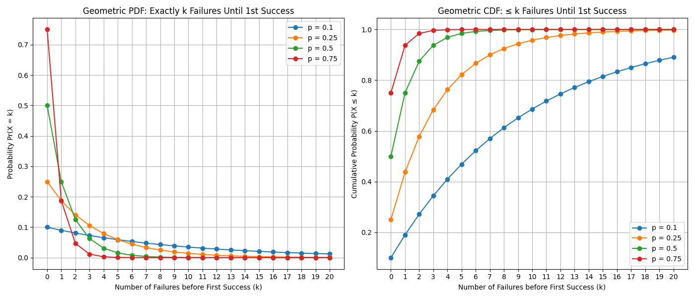
You can generate the graph above with make geometric_pdf_vs_cdf.py
Total Rewards: Expected Value Calculation for Dishonest Supplier Before Penalty
This represents the Supplier's earnings before the penalty is applied.
If the Supplier chooses to leave the network at this point in time, it will have successfully gamed the system.
Expected Penalty: Slashing amount for Dishonest Supplier
The penalty is a fixed amount S when caught.
Total Profit: Expected Value Calculation for Dishonest Supplier AFTER Penalty
Honest Supplier: Calculating the Expected Value
-
Expected Rewards per Claim:
-
No Penalties: Since the honest Supplier always provides valid Proofs when required, they avoid penalties.
-
Expected Profit for Honest Supplier (1 Claim):
Setting Parameters to Deter Dishonest Behavior
To deter dishonest Suppliers, we need:
Substituting the expected values:
Since q = 1 -p, we can simplify the inequality to:
Solving for Penalty S
However, since p is between 0 and 1, 1 - 2p can be negative if p > 0.5.
To ensure S is positive, we consider p ≤ 0.5.
Alternatively, to make the penalty effective, we can set:
This ensures that the expected profit for dishonest Suppliers is 0 or negative:
Example Calculation
Assume:
- Reward Per Claim:
R = 10 - ProofRequestProbability:
p = 0.2 - Probability No Proof Requested:
q = 0.8
Calculate the expected profit for a dishonest Supplier:
-
Expected Number of False Claims Before Getting Caught:
-
Expected Total Rewards:
-
Penalty:
-
Expected Profit:
The dishonest Supplier has an expected profit of 0, making dishonest behavior unattractive compared to honest behavior, which yields a profit of R = 10 units per Claim without risk of penalty.
Generalizing the Penalty Formula
To ensure that dishonest Suppliers have no incentive to cheat, set the penalty S such that:
This makes the expected profit for dishonest behavior 0:
TODO_IN_THIS_PR, incorporate feedback from ramiro:
This value will provide the attacker no expected return, but also no penalty.
In fact, the expected cost of sending an attack is 0 POKT.
An attacker can keep sending claims to the network because at the end of the day s/he will not lose money. This enables spam in the network.

We can model this using the quantile function (or "percent point function"), the inverse of the CDF.
Sadly I found no closed form for the geometric function (because it is a step function), but we can calculate it easily (is a really small iterative process).

For example, to be sure that in 95% of all the attacks the attacker is punished (or breaks even in a marginal number of samples), we should set the slash amount (S) approx 3x from what you use here (~6K POKT for the numbers in this example).
Doing this will penalize the attacker/spammer with an average of 4K POKT per attack try.

If you want I can create small notebook with the procedure and simulation.


Some notes:

The CDF of the E(Geom(p=0.01)) is 63%, meaning that 37% of all attacks result in net profit (some very large).
I use 95% in the example but this can be less, like 75%, resulting in lower S and hence lower min stakes while adding net loss to the attacker). Any value above 63% will result in net loss for the attacker.
Source: https://gist.github.com/RawthiL/9ed65065b896d13e96dc2a5910f6a7ab
Considering false Claim Variance
While the expected profit is 0, the variance in the number of successful false
Claims can make dishonest behavior risky. The Supplier might get caught earlier than expected,
leading to a net loss.
TODO_IN_THIS_PR: Incorporate this from Ramiro: Variance works both ways, hence my previous comment. This can be a justification for changing the calculation of S as I suggest. This is because the attacker might not be caught until much later and result in a net profit.
Crypto-economic Analysis & Incentives
Impact on Honest Suppliers
Honest Suppliers are not affected by penalties since they always provide valid Proofs when required. Their expected profit remains:
TODO_IN_THIS_PR: Honest faulty suppliers will also be affectd and peanlized, which was not an issue before.
What about non-malicious faults (e.g. network outage)? In this case, I would argue that there's definitely a potential for impact on honest suppliers. Do you see it differently? Is it worth mentioning that possibility here?
Impact on Dishonest Suppliers
Dishonest suppliers must contend with substantial penalties that erase their anticipated profits, coupled with a heightened risk of early detection and ensuing net losses.
Furthermore, the inherently probabilistic nature of Proof requests introduces additional uncertainty, making dishonest behavior both less predictable and more costly.
Analogs between Model Parameters and onchain Governance Values
Parameter Analog for Penalty (S)
tl;dr S = Supplier.MinStake
The penalty S is some amount that the protocol should be able to retrieve from the Supplier.
In practice, this is the Supplier.MinStake parameter, which is the amount a Supplier
always has in escrow. This amount can be slashed and/or taken from the Supplier for misbehavior.
Parameter Analog for Reward (R)
tl;dr R = Proof.ProofRequirementThreshold
In practice, the reward for each onchain Claim is variable and a function of the amount of work done.
For the purposes of Probabilistic Proofs, we assume a constant reward of R per Claim
because any reward greater than ProofRequirementThreshold requires a proof and
short-circuits this entire document.
Therefore, R can be assumed constant when determining the optimal p and S.
TODO_IN_THIS_PR: Explain p
Considerations during Parameter Adjustment
TODO_IN_THIS_PR: Add a mermaid diagram for this.
By tweaking p and S, the network can:
- Increase the deterrent against dishonest behavior.
- Balance the overhead of Proof verification with security needs.
Considerations:
- Lower
preduces the number of Proofs required --> improves scalability --> requires higher penalties. - Higher
Sincreases the risk for dishonest Suppliers --> lead to social adversity from network participants.
TODO_IN_THIS_PR: Explain how How does a high slashing penalty increase the risk of dishonest suppliers?
Selecting Optimal p and S
TODO_IN_THIS_PR: Add a mermaid diagram for this.
To select appropriate values:
-
Determine Acceptable Proof Overhead (
p):- Choose
pbased on the desired scalability. - Example:
p = 0.1for 10% Proof submissions
- Choose
-
Calculate Required Penalty (
S):- Ensure
Sis practical and enforceable. - Use the formula:
- Ensure
-
Assess Economic Impact:
- Simulate scenarios to verify that dishonest Suppliers have a negative expected profit.
- Ensure honest Suppliers remain profitable.
To illustrate the relationship between p, S, see the following chart:
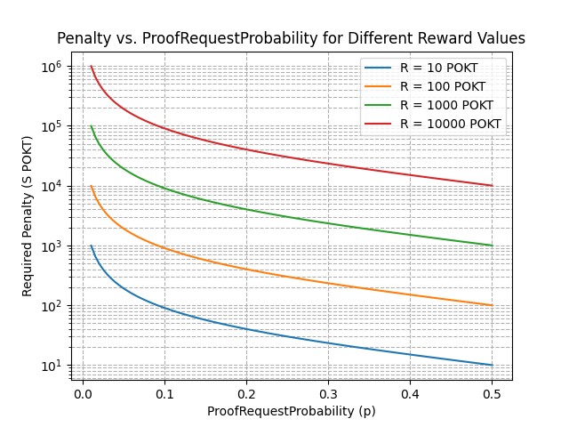
You can generate the graph above with penalty_vs_proof_request_prob.py
Considerations for Proof.ProofRequirementThreshold an ProofRequirementThreshold
- Threshold Value: Set the
ProofRequirementThresholdlow enough that most Claims are subject to probabilistic Proof requests, but high enough to prevent excessive Proof submissions. - Short-Circuiting: Claims above the threshold always require Proofs, eliminating the risk of large false Claims slipping through.
ProofRequirementThreshold should be as small as possible so that most such that
most Claims for into the probabilistic bucket, while also balancing out penalties
that may be too large for faulty honest Suppliers.
Normal Distribution
Assume Claim rewards are normally distributed with a mean μ and standard deviation σ.
Ideally, we would choose 2σ above the Claim μ such that 97.3% fall of all Claims require a Proof.
Non-Normal Distribution
In practice, rewards are not normally distributed, so we can choose an arbitrary value (e.g. p95)
such that 95% of Claims fall into the category of requiring a proof.
Considerations for ProofRequestProbability (p)
See Pocket_Network_Morse_Probabilistic_Proofs.ipynb for more details from Morse, supporting the fact that the majority of the block space is taken up by Proofs.
The number of on-chain relays (proofs) required by the network scales inversely to ProofRequestProbability. For example:
ProofRequestProbability= 0.5 -> 2x scaleProofRequestProbability= 0.25 -> 4x scaleProofRequestProbability= 0.1 -> 10x scaleProofRequestProbability= 0.01 -> 100x scaleProofRequestProbability= 0.001 -> 1000x scale
Maximizing Pr(X<=k) to ensure k or less failures (Supplier escapes without penalty)
When selecting a value for p, our goal is not to maximize Pr(X=k), but rather
maximize Pr(X<=k) to ensure k or less failures (Supplier escapes without penalty).
This does not affect the expected reward calculations above, but gives a different perspective of what the probabilities of success and failure are.
Conclusions for Modeling
By modeling the attack using a geometric distributions and calculating expected values, we can:
- Determine
R = ProofRequirementThresholdusing statical onchain data. - Manually adjust
p = ProofRequestProbabilityto adjust scalability. - Compute
S ≤ SupplierMinStaketo deter dishonest behavior. - Determine the necessary penalty
Sto deter dishonest behavior. - Ensure that honest Suppliers remain profitable while dishonest Suppliers face negative expected profits.
This approach allows the network to scale by reducing the number of on-chain Proofs while maintaining economic (dis)incentives that deter dishonest behavior.
Morse Based Value Selection
As of writing (October 2024), Shannon MainNet is not live; therefore, data from Morse must be used to approximate realistic values.
Selecting ProofRequirementThreshold
Choose R = 20 since it is greater than p95 of all Claims collected in Morse.
Units are in POKT.
See the original proposal from Morse available in probabilistic_proofs_morse.md and Pocket_Network_Morse_Probabilistic_Proofs.ipynb for supporting data.
Calculating p: ProofRequestProbability
Choose p = 0.01 to ensure high scalability.
Calculating S: ProofMissingPenalty
TODO_IN_THIS_PR: Above Threshold Attack Possibility
above threshold attacks possibilities.
We should investigate above threshold attacks possibilities.
Supplier adds fake serviced relays to the SMT. Submits the claim. If the closest proof corresponds to a: a. Fake relay -> Do not submit the proof and face slashing. b. Legit relay -> Submit the proof and be rewarded for fake relays.
This is interesting, you talk about inflating the tree with fake relays. I think that the effect will be a reduction of the catch probability that is proportional to the fake relays ratio. Supose that you inflate your tree by a X%, then you have a a chance of being requested a proof given by ProofRequestProbability and a X/100 chance that the requested proof is a fake relay. I think that in practice this can be modeled as a reduced ProofRequestProbability, so we can add a security factor there.
Future Work
-
Attack Vector: Account for the fact that a Supplier could be in multiple sessions at the same, so either:
- The number of sessions a supplier is in will need to be limited
- The minimum stake amount will need to be significantly higher than the penalty to enable slashing across multiple sessions at once
- It could be a multiple of its provided services count.
-
Optimal Reward Value: Evaluating onchain Shannon data to determine the optimal value for
R -
Closed Feedback Loop: Having
pdynamically adjust onchain as a function of onchain data without intervention from the DAO / PNF. -
Reviewing, comparing & contributing to external literature such as: